Eden Quick
Start
[Revised on 20 May
2004]
Eden is a very well-written and well-documented program, but it is
perhaps easiest to learn how to run it by following an example.
When you install eden, you will have a directory in /usr/local/eden
or /sw/eden (or wherever you installed it) called eden/example.
This uses crambin and is a very good place to start. If you
want to use that, I suggest first copying everything in the example
directory into a directory under your home directory.
What follows is a different, perhaps simpler, example, taken from
real life, and ideally this should be something anyone could do,
not just a crystallographer. The idea is that you see an
interesting structure in the literature, and you download the
coordinates and Fobs from the pdb and then you calculate an eden
map to see the density for yourself. This is a good way to
confirm the veracity of the structure, and to test it using a
perturbation/randomization test available in eden.
I'll use as an example an interesting structure recently published
in Science in which a pentacoordinated oxyphosphorane is observed
at high resolution. There has been considerable debate over
whether such a structure could exist even as a transient
intermediate vs. a metastable transition-state. No one had
ever suggested such a thing could hang around on crystallographic
time scales, so this is really quite interesting. I wanted to
convince myself it was right; and by calculating maps in Eden, I am
convinced. Eden makes maps in a way that is probably minimally
biased by the starting model. Here is how I did it:
1.
Download the pdb and Fobs from the protein data bank.
Move 1O08.pdb and r1o08sf.ent into a new directory where
you want to work. Copy the file eden/tools/awk_pdb into
your working directory.
a.
Reformat the pdb file like this:
% awk
-f awk_pdb < 1O08.pdb >
penta.pdb
b. Reformat the
Fobs like this:
1. Cut
out all the leading crap until the line of the first reflection, as
well as the last line in the file.
2. Reformat it as
an xplor (CNS) data file. I did this using xdldataman (input
as free format). I saved the file in xplor format and called
it pentacoord.fobs and its first three lines look like
this:
INDEX= 0 0 4 FOBS= 73.150 SIGMA= 1.340
INDEX= 0 0 16 FOBS= 99.300 SIGMA= 1.540
INDEX= 0 0 18 FOBS= 51.370 SIGMA=
0.840
2. Make an input
file that looks like this: (I called mine
pentaphos.inp)
TITLE
BETA-PHOSPHOGLUCOMUTASE
CELL
36.939 54.297 104.680 90.00
90.00 90.00
SYMMETRY
P212121
INPUT_RES
1.20
MODE
correction
FSCALE
1.0
ANOM
False
3. Use the pdb
file to calculate fcalcs in Eden:
Note:
Difference fouriers don't exist in the world of direct-space
map refinement, but you can chop out part of the pdb file
corresponding to a bit of the structure in question (which is
equivalent to having an incomplete model) and then you can run eden
in the "completion" rather than the "correction" mode
by changing the input file. The density that appears for the
missing part of the structure in general will be only about 1/3
as strong as that for which the model atoms are present, so
please be aware that you will have to contour your map lower
(0.6 to 0.4 * rmsd) to see the density for the missing part of the
structure clearly. In the present example I don't have you do
this, but omitting the pentacoordinated phosphate atoms would be
the more rigorous way to do
this.
% eden -v tohu pentaphos penta.pdb
Note that you give eden
the input file (in this case pentaphos.inp) without the suffix and
then the pdb file. You will get output that looks like
this:
Thu May 20 11:26:52 2004
tohu, Version 4.3
**********************************************************
WARNING: Tohu is a slow
substitute for other programs that
calculate structure
factors from PDB information. It uses
B values, but assumes
point atoms. However, it produces
structure factors on an
absolute scale without any further
manipulation.
**********************************************************
Reading file
pentaphos.inp
Pdb file contains:
1106 C
atoms, 6570 electrons
285 N
atoms, 1995 electrons
821 O
atoms, 6536 electrons
1 MG
atoms, 12
electrons
2 P
atoms, 30
electrons
3 S
atoms, 48
electrons
Total: 2218 atoms.
15191
electrons
Total zsq : 107035
total pdb
electrons in unit cell 60764 corresponds to Fobs(000) ~
83000
Matthews' coefficient is 3.45524
and protein fraction is 0.689084.
Max. # of unique and non-unique reflections: 371376 383776
Generating unique reflections only.
Finished calculating 10000 structure factors
... <snip> ...
Finished calculating 370000 structure factors
Writing penta.fcalc file
A log of this run has been written to tohu1.log
Thu May 20 11:54:03
2004
% eden -h tohu explains how this works.
You will get a popup wish window. This is the slowest
part in Eden. If you have a big cell or high resolution data
you might be better off doing this in CNS or with SFALL in
CCP4.
4. Apodize and
scale the data.
Apodization
is something NMR spectroscopists do more than crystallographers,
but very briefly, it means "smearing out" the data slightly so that
the refinement will be more well-behaved. Read the
documentation for a better description. First we apodize the
fcalcs produced by eden tohu, and then we will attempt to put the
apodized fobs on an absolute scale. We do so with
eden
apodfc and
eden
apodfo as follows:
a.
Apodize the fcalcs:
Issue the
command
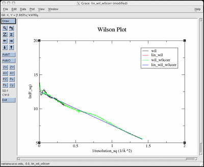
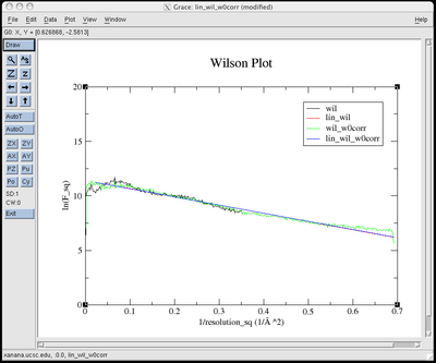
% eden -v -g
apodfc pentaphos penta.fcalc
Here is a screenshot of
the pop-up graph that appears when you supply the (optional) -g
flag and have grace installed:
Dismiss the grace window
when you are done looking at the plot and eden will
continue.
eden -v -g apodfc pentaphos penta.fcalc
Thu May 20 12:28:47 2004
apodfc, Version
4.3
Reading file
pentaphos.inp
Linearization limits are (3.5, 0.05) A.
Apodization resolution = 1.2 A.
742521 Fcalc entries are valid,
Fcalc(0,0,0) = (60764, 0)
# of bins set to 710, average bin size is 0.002.
Doing calculation
without correction for proteins ...
The average crystallographic B factor is 9.80745 Asq,
corresponding to a resolution of 0.919231 A.
The data should be smeared using a target B factor of
16.7136.
Standard deviation of wilson curve (uncorrected) with
respect
to its linearized version is 0.179644.
Redoing calculation
with correction ...
The average crystallographic B factor is 9.88273 Asq,
corresponding to a resolution of 0.922752 A.
The data should be smeared using a target B factor of
16.7136.
Standard deviation of wilson curve (corrected) with respect
to its linearized version is 0.174195.
Proposed plot is
uncorrected - ok [y/n]? y
Using original Wilson plot (apodized).
The new average crystallographic B factor is 16.7136
Asq.
The crystallographic B factor correction is 6.90613
Asq.
Writing penta_apo.fcalc
PLEASE NOTE:
The Wilson file 'penta.fcalc_wil' should be used for scaling
your fobs.
A log of this run has been written to apodfc2.log
Thu May 20 12:35:54
2004
b. Apodize and scale the Fobs.
First we need
the estimate a value for the (unobserved) F(000) (tohu
reported
Fobs(000) ~
83000.
above) and we estimate
sigmaF(000) as the square root of 0.1 * F(000),
i.e,
SigF(000) ~ 91.
Then put that into the
first line of pentacoord.fobs and issue
% eden -v -g
apodfo pentaphos pentacoord.fobs
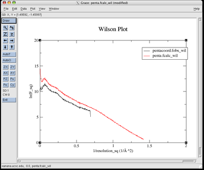
You will get a grace
window with a wilson plot. When you dismiss that window, it
will ask if the proposed plot is uncorrected. Answer yes or hit the
return key. Then you will see the following prompt, to which
you should answer yes and provide the fcalc Wilson Plot file
name:
Writing
pentacoord_apo.fobs
Scale? - y or n:
y
Enter name of file
containing fc Wilson data: penta.fcalc_wil
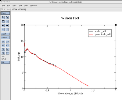
You will see before and
after plots that look like this:
eden -v -g apodfo pentaphos
pentacoord.fobs
Thu
May 20 12:50:04
2004
apodfo, Version
4.3
Reading file
pentaphos.inp
Linearization
limits are (3.5, 0.05)
A.
Apodization
resolution = 1.2
A.
56675
(expanded to 217590) out of 56675 Fobs entries read
in;
Fobs(0,0,0)
= 83000, sigma =
91
# of
bins set to 347, average bin size is
0.002.
Sigma
apodization coefficients are 0.27665 and
0.000289082
Doing calculation without correction for proteins
...
The
average crystallographic B factor is 15.0258
Asq,
corresponding
to a resolution of 1.1378
A.
The data
should be smeared using a target B factor of
16.7136.
Standard
deviation of wilson curve (uncorrected) with
respect
to its linearized version is
0.232316.
Redoing calculation with correction
...
The
average crystallographic B factor is 14.9343
Asq,
corresponding
to a resolution of 1.13433
A.
The data
should be smeared using a target B factor of
16.7136.
Standard
deviation of wilson curve (corrected) with
respect
to its linearized version is
0.211667.
Proposed plot is uncorrected - ok [y/n]?
y
Using
original Wilson plot
(apodized).
The new
average crystallographic B factor is 16.7136
Asq.
The
crystallographic B factor correction is 1.68777
Asq.
Writing
pentacoord_apo.fobs
Scale? - y or n:
y
Enter name of file containing fc Wilson
data
from the end of your Apodfc run:
penta.fcalc_wil
Proposed
value for fscale is
1.70486
A log of
this run has been written to
apodfo5.log
Thu May
20 12:55:32 2004
Your apodized data,
which is not yet on an absolute scale, is now in the
file:
pentacoord_apo.fobs
You must manually input
the scale factor as shown below in step 6.
We are now finally ready to do a map
calculation.
5. Run eden back
to get the first-order model-based approximation to the
map:
If you first
type eden -h
back, a wish window will display this:
"Back
estimates electron densities from a set of calculated diffraction
patterns with phases. . . . One purpose of this calculation is to
provide Eden with a "known" map, whose values may serve to set
initial bounds on the
solver."
That is what we are
doing now. Issue
% eden -v back
pentaphos penta_apo.fcalc
The initial map is written to a binary file called
pentaphos_back.bin
6. Run eden
solve:
a. Edit
the input file to include two more lines. These tell eden to
use the scaled, apodized fobs and the "known" fcalc map. Also
be sure to set the scale factor explicitly as shown in red.
TITLE
BETA-PHOSPHOGLUCOMUTASE
CELL
36.939 54.297 104.680 90.00
90.00 90.00
SYMMETRY
P212121
INPUT_RES
1.20
MODE
correction
FSCALE
1.7
ANOM
FALSE
FO_FILENAME
pentacoord_apo.fobs
MD_FILENAME
pentaphos_back.bin
b.
Issue the command
% eden -v solve
pentaphos
This takes awhile to run. It generates output that looks like
this:
Command
line: eden -v solve pentaphos
Thu May 20 13:09:28 2004
solve, Version
4.3
Reading file
pentaphos.inp
Dump of pentaphos.inp follows:
TITLE
BETA-PHOSPHOGLUCOMUTASE
CELL
36.939 54.297 104.680 90.00
90.00 90.00
SYMMETRY P212121
INPUT_RES 1.2
MODE
correction
FSCALE
1.7
ANOM
FALSE
FO_FILENAME pentacoord_apo.fobs
MD_FILENAME pentaphos.bin
End of pentaphos.inp dump.
Unit cell measures 36.94 by 54.30 by 104.68
Angstrom
Alpha = 90.00, beta = 90.00, gamma = 90.00
degrees
Scale factor for converting el/A^3 to el/grid pt is 0.295864
Symmetry is P212121.
Input resolution is 1.2 Angstrom.
Gridding resolution is 0.84 Angstrom, eta is 0.6
Input unit cell partitions are 44.0 by 64.6 by 124.6
Actual unit cell partitions are 44 by 64 by 126
Average resolution in Angstrom is dr = 0.8396
Partition errors (%) with respect to the average resolution
in a, b and c are 0.00917511, -1.03619, and 1.05996.
Eden grid is body-centered.
The anomalous data flag is not set.
Run summaries will be written to history.
******************************************************
This is an Eden run in
correction mode.
There are no Np
constraints in the cost function.
******************************************************
BETA-PHOSPHOGLUCOMUTASE
Observed structure factors will be read from
pentacoord_apo.fobs
Sigmas will be used for weighting
Data scaling factor is 1.7
Structure factors will be calculated from pentaphos.bin
Stop getsol if df/dx is reduced to 0.03 of its initial value
Starting physical space model will be read from pentaphos.bin
Relative weight for Nhkl space is 1
Approximate (underestimated) memory requirements in Mbytes:
Physical space: 65.3, Reciprocal space: 165, Total:
230.
Setting up initial arrays ...
Begun making FFT plan ...
... Finished making FFT plan.
Reading fobs file
... for native
1/d-squared shell limit is 0.41508, based on data
217590 (expanded to 217590) out of 217590 Fobs entries read
in;
Fobs(0,0,0) = 83000, sigma = 91
Sigma ranges
For native:
Sigma range is 0.415971 - 40.4209
Hkl weight normalization factor = 1.4157
Reading model electron map ...
Nptotal = 709632, Npextended = 709632
The volume coefficient: V/(2pi*eta*drsq)^3/2 = 48463.1
Generating fcalc file.
Fc reflections thrown out: 525089
F Percentages, Fo and Fc counts for fractions of 1/d-squared
(000)
1/8
1/4 1/2
Remainder Overall
res
(A)
> 3.4 3.4- 2.4 2.4-
1.7 1.7- 1.2
all
% F 0.327457 14.7857
21.9706 33.6183
29.2979 100
# Fo
1
9985
20307 55893
131400 217586
# Fc in
1
9985
20307 55893
131400 217586
# Fc out 0
1198
356
1788
32115 35457
max #
1 11950
21447 59216
166609 259223
This problem has 217590 equations, 709632 unknowns
R factors for fractions of 1/d-squared
(000)
1/8
1/4 1/2
Remainder Overall
resol
(A)
> 3.4 3.4- 2.4 2.4-
1.7 1.7- 1.2
all
0.326806 0.425757 0.442269
0.455249 0.491043 0.458103
Percentages of Fcalcs
within sigma intervals of Fobs:
interval:
1
2
3
4 outliers
% native:
1.43895 1.15815
1.30659 1.35347 94.7428
% for Gaussian: 68.2689
27.181 4.28005 0.263645
0.00633425
Goodness-of-fit: chisq = 828.735, robust chisq = 95.8647
Thu May 20 13:09:39 2004
Applying holographic reconstruction -
iteration # 1
Stopping criterion for the (hkl) cost function is 2.2e+05
Using the original hkl cost function.
Initial standard deviation = 11.2851
Initial value of the (hkl) cost function is 1.8e+08
df/dx went down enough, 128 funct calls
Sum of recovered electrons in this iteration is 59038.3
Standard deviation before symmetrization = 2.04957
The rms fractional distance between original and symmetrized arrays
is 2.78001e-10
Standard deviation after symmetrization = 2.04957
Cumulative sum of recovered electrons is 59038.3,
Variance of electrons/voxel for this iteration is 0.205891
Total electrons (starting model plus recovered): 169163
Analysis of
electron densities:
Range is (0, 7.1791) el/voxel, (0, 24.2649) el/cubA.
Distribution of electron densities:
Range (el/cubA) %
< 0.1:
31.38
0.1 - 0.2: 9.67
0.2 - 0.3: 7.30
0.3 - 0.4: 5.78
0.4 - 0.5: 4.76
0.5 - 0.6: 4.05
0.6 - 0.7: 3.65
0.7 - 0.8: 3.22
0.8 - 0.9: 2.96
> 0.9:
27.23
R factors for fractions of 1/d-squared
(000)
1/8
1/4 1/2
Remainder Overall
resol
(A)
> 3.4 3.4- 2.4 2.4-
1.7 1.7- 1.2
all
1.03811 0.0371284 0.0288496 0.0376395
0.151755 0.0723422
Percentages of Fcalcs
within sigma intervals of Fobs:
interval:
1
2
3
4 outliers
% native:
42.9447 19.2592
7.99351 5.35919 24.4433
% for Gaussian: 68.2689
27.181 4.28005 0.263645
0.00633425
Goodness-of-fit: chisq = 25.2826, robust chisq = 9.20989
Current value of the (hkl) cost function is 6.0e+06
...<snip> ...
Thu May 20 15:21:27 2004
Applying holographic reconstruction -
iteration # 9
Stopping criterion for the (hkl) cost function is 2.2e+05
Initial standard deviation = 0.423306
Too many iterations in Getsol. The solver is STUCK - please
re-examine your input!
Sum of recovered electrons in this iteration is -1974.4
Standard deviation before symmetrization = 0.408877
The rms fractional distance between original and symmetrized arrays
is 5.94666e-05
Symmetrization changed 26 out of 177408 asym. unit elements
by more than 10.000 %
of the average.
Standard deviation after symmetrization = 0.408876
Cumulative sum of recovered electrons is 33725.1,
Variance of electrons/voxel for this iteration is 0.0861696
Total electrons (starting model plus recovered): 143850
Analysis of
electron densities:
Range is (0, 13.4375) el/voxel, (0, 45.4177) el/cubA.
Range (el/cubA) %
Subrange (el/cubA) %
< 0.1:
67.76 0.00 -
0.01: 59.68
0.1 - 0.2:
3.19 0.01 -
0.02: 2.10
0.2 - 0.3:
2.15 0.02 -
0.03: 1.38
0.3 - 0.4:
1.76 0.03 -
0.04: 1.01
0.4 - 0.5:
1.46 0.04 -
0.05: 0.85
0.5 - 0.6:
1.31 0.05 -
0.06: 0.68
0.6 - 0.7:
1.22 0.06 -
0.07: 0.63
0.7 - 0.8:
1.12 0.07 -
0.08: 0.53
0.8 - 0.9:
1.13 0.08 -
0.09: 0.49
> 0.9:
18.90 0.09 -
0.10: 0.41
R factors for fractions of 1/d-squared
(000)
1/8
1/4 1/2
Remainder Overall
resol
(A)
> 3.4 3.4- 2.4 2.4-
1.7 1.7- 1.2
all
0.733132 0.00208563 0.00138599 0.00157887 0.00822229
0.00595333
Percentages of Fcalcs
within sigma intervals of Fobs:
interval:
1
2
3
4 outliers
% native:
99.0128 0.924679 0.056069 0.00459582
0.00183833
% for Gaussian: 68.2689
27.181 4.28005 0.263645
0.00633425
Goodness-of-fit: chisq = 0.0607023, robust chisq = 0.058839
Final value of the (hkl) cost function is 2.4e+05
Overall R factor changed from 0.458103 to 0.00595333
Total number of solver search directions was 2481
Total number of cost function calls was 4930
Thu May 20 16:03:38 2004
The output map is in
binary form in the file pentaphos.bin. You can make an xplor
map by typing this:
% eden regrid
pentaphos pentaphos 2
The map will be named
pentaphos_2.map
To display it in pymol, I will rename it to
penta.xplor
Here is a pymol script
to display the results:
load
closeup_penta.pdb, closeup
load
1O08.pdb
load
penta.xplor, map1
isomesh
msh0,map1,3.5,closeup,0.1,1,2.0
color
blue,msh0
isomesh
msh1,map1,4.5,closeup,0.1,1,2.0
color
white,msh1
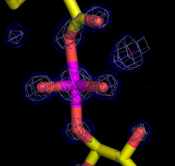
Here is a
snapshot of the eden density at the pentavalent phosphate as
displayed in
pymol:
Note that if you are using eden to perform the functional
equivalence of a difference Fourier in completion mode (i.e., you
left the atoms in question out of the pdb file or changed their
occupancy to zero), you will have to contour the map much lower,
i.e., around 0.3 rms, in order to see the density at a "normal"
level. This is essentially an artifact that is a consequence
of eden's real-space map calculation. There is no 3Fo-2Fc map
equivalent in eden.
